Link to Project Repository
Contents
Introduction
A few months ago, I chanced upon a video that demonstrated a commercial Furuta Pendulum design used to teach control theory at the university level. As someone who is always itching to try a new reinforcement learning (RL) project, this felt like the perfect challenge to apply RL to a hardware system from scratch!
What is it?
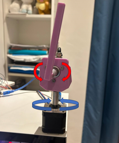 A Furuta Pendulum is a control problem which involves a pendulum that swings in the vertical plane (as annotated with red arrows above) driven by a motor shaft in the horizontal plane (as annotated with blue arrows). The goal of the robot is to swing the pendulum to the upright vertical position (an inverted pendulum) and to keep it balanced in that position for as long as possible.
Project Overview
This project involved building the hardware and software components of the robot from scratch and integrating them into one coherent system. The project can largely be split into 3 major design components:
- Robot Design: The physical hardware of the robot and the Arduino code for sending the robot’s raw motor and pendulum positions, while receiving and executing control instructions from the PC.
- Robot Environment: The environment that the RL model interacts with to control the robot. This “middleman” between the robot and model serves to translate the raw data sent between the two to ensure that the interaction is seamless.
- RL Model: The model makes the control decisions for the robot and seeks to optimise the reward calculated by the environment by continuously fine tuning its policy.
RL Model
The bread and butter of designing an RL model is building its action space, observation space and reward function. Essentially, RL models receive observations of the environment’s state (observation space) and choose the best decision from the action space to interact with the environment to maximise the reward generated by the environment.
 Pendulum environment from OpenAI. Credit: gymlibrary.dev (link below)
This was difficult to engineer from scratch, and I looked at similar experiments such as the pendulum problem and cartpole problem from OpenAI gym for inspiration. I also designed the reward function based on existing furuta pendulum designs such as the original Quanser Qube (the robot from the video i saw).
Listed below are the relevant variables that were selected for the different spaces and reward function:
- $\theta$: angular position of pendulum. 0 at the top and normalised between $[-\pi,\pi]$.
- $\dot{\theta}$: angular velocity of pendulum. Experimentally bounded between $[-10,10]$, then normalised to between $[-2, 2]$.
- $\alpha$: motor position (measured in steps instead of angle). Steps range physically limited to 90° left and right or $[-200, 200]$ step range. However, observation space spans further between $[-300, 300]$ to account for the motor exceeding the limit slightly. The range is then normalised between $[-3,3]$.
- $\dot{\alpha}$: motor velocity (steps per second). Experimentally bounded between $[-4, 4]$, then normalised to between $[-1, 1]$
- $\ddot{\alpha}$: motor acceleration (steps per second squared). Control input into the system. Bounded between $[-20000,20000]$ and normalised between $[-2, 2]$.
For these variables, normalisation is critical, as it improves training stability and ensures that the variables are scaled relative to each other.
Action Space
$\left[\ddot{\alpha}\right]$
The action space is the simplest to design. Taking inspiration from the OpenAI pendulum problem which uses torque as an action input to swing the pendulum up, I decided to use the motor acceleration as the action input to the robot. The input to the robot was thus an acceleration value between -20k to 20k.
This could be represented as a discrete action space of 40k possible actions. However, I noted that a large discrete action space was not necessarily efficient and lacked context in terms of the closeness of neighbouring acceleration values that a continuous action space could better describe.
Hence, I decided on a normalised continuous action space between -2 to 2, mapping the action input to the correct motor acceleration value.
Observation Space
$\left[\cos{\theta}, \sin{\theta}, \dot{\theta}, \alpha, \dot{\alpha}\right]$
The observation space took inspiration from the pendulum problem from OpenAI and from the Quanser Qube code. Essentially, we are interested in reporting the motor position and pendulum angular position to the model, along with their respective velocities. The choice for using $\cos{\theta}$ and $\sin{\theta}$ instead of just $\theta$ was due to reportedly better convergence in results. This can be attributed to the fixed range of $[-1, 1]$ and providing both gives more information about the state.
Reward
$\gamma-\left(\theta^2+C_1\times\dot{\theta}^2+C_2\times\alpha^2+C_3\times\dot{\alpha}^2+C_4\times\ddot{\alpha}^2\right)$
$\gamma$: reward offset value (offset) to ensure that reward is always positive.
The reward function was derived from the Quanser reward function, where it is a negative cost function that mainly punishes for when the pendulum is not upright. It also penalises motion in the pendulum and motor to nudge the robot to converge towards a policy that minimises movement and jitter when trying to balance the pendulum.
However, with a negative cost function, the reward is $-\inf$ to $0$, where episodes with early termination would generate an unfairly higher reward (because they would accumulate smaller negative reward). Hence, the reward offset aims to prevent this issue. Constants $C$ are used to adjust the reward function weightage and are defined in the /conf/config.yaml.
Termination and Truncation
Truncation: Training episodes for the model must be truncated, as there is no winning terminal condition for this environment. Hence, we set the episode length to be 500 timesteps, a good balance between giving the robot enough time to explore each episode and chopping up the entire training into enough episodes for the robot to finetune and learn from.
Termination: The only terminal state for this environment is when the robot exceeds the allowed range of motion (more than 90° left or right from the zero position). We ensured above that early termination due to the robot leaving the allowed range is naturally “punished”, by restricting its maximum reward per episode if it chooses to terminate early.
Model Selection
Since the observation space was continuous, I decided to work with both Proximal Policy Optimization (PPO) and Soft Actor-Critic (SAC) models, finding greater success with SAC. The models were both deployed using Stable-Baselines3 (SB3) and their weights were managed using the hydra module.
SAC is a much more sample efficient policy compared to PPO, which can be credited to its off-policy algorithm vs on-policy in PPO. This could explain why the SAC model began seeing better results much earlier than PPO.
One of the critical parameters I set for both models was to enable Generalised State Dependent Exploration (gSDE), as raised in this video. This is critical for real-life robotic applications, which allows for smoother policies that can be applied realistically to physical systems that cannot respond instantaneously to Gaussian noise inputs.
Robot Design
Now that we know what data we require to receive and send to the robot for the RL model to train on, we can move on to designing the robot proper.
Hardware Design
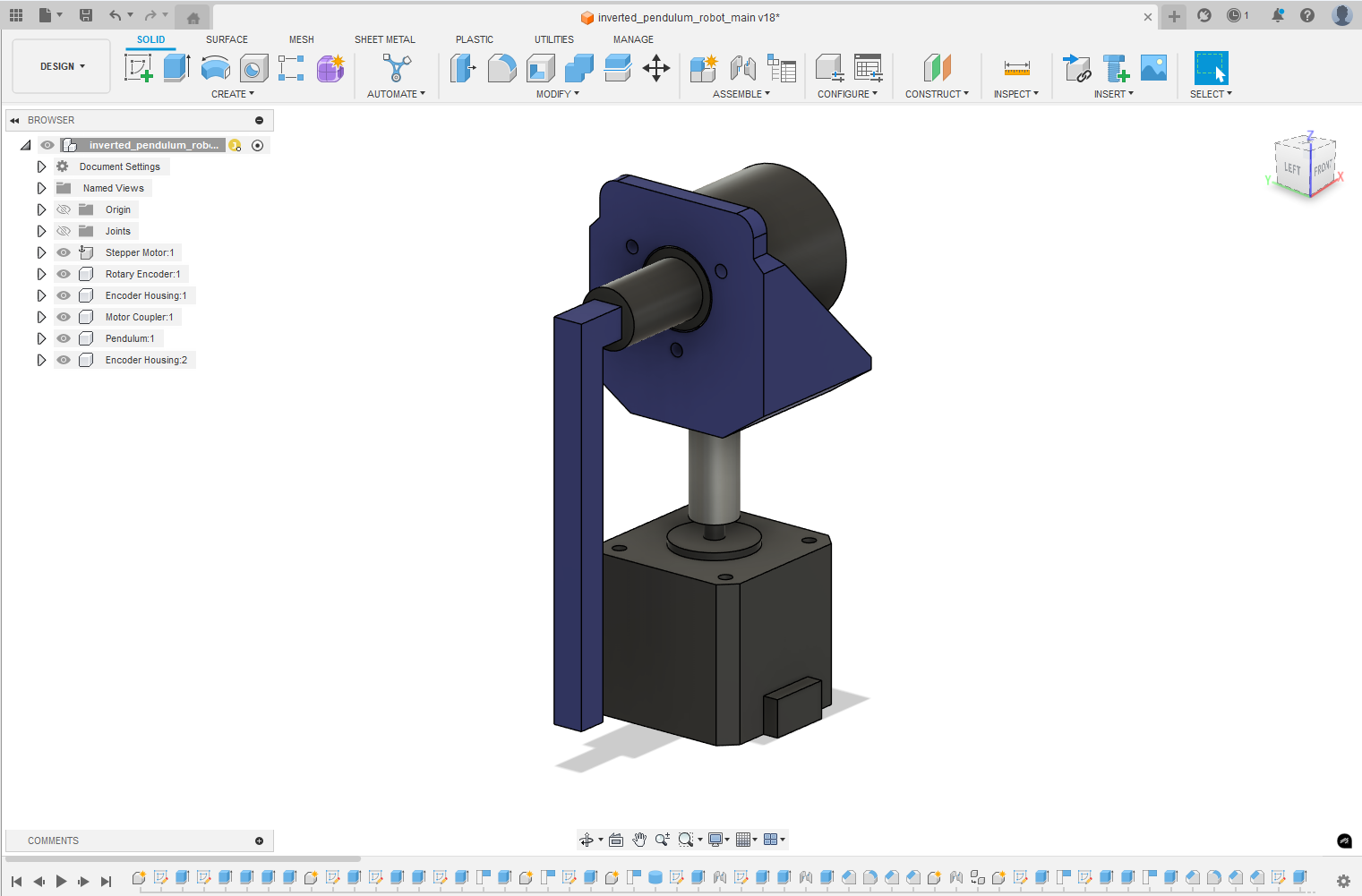
Visit my repo to view the parts list for this project and to see the Fusion 360 CAD design.
The hardware design for this project was fairly straightforward. The robot was essentially just a rotary encoder cleverly connected to a motor using rigid couplers and 3D printed parts. However, since this was a complex control problem, it was important that the robot could achieve precise movements and report accurate positioning data.
Motor
I decided on a stepper motor, as it provides a high precision and high torque solution. A stepper motor was chosen in favour over a servo, simply due to cost (especially for a servo that can rotate 360°).
An average stepper motor provides a step resolution of around 1.8°. However, I set the motor on a quarter-step setting to get a step resolution of around 0.45°.
The stepper motor also allowed me to return the robot to a home position consistently. This was critical for resetting the robot environment after each training episode.
Rotary Encoder
A broad distinction for rotary encoders is between incremental encoders and absolute encoders. Incremental encoders measure the change in position, rather than reporting the actual absolute position.
I found cheap high precision incremental encoders online, and decided to work with them. Incremental encoders allowed me to accurately report angular velocity (since it measures change).
However, since the absolute position of the encoder is not persistent, the encoder had to be zeroed at the vertical down position before every run.
 Credit: dynapar.com (link below)
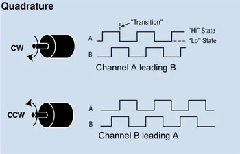
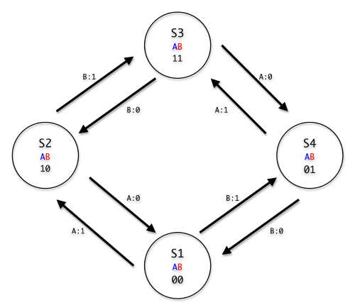
I also needed to know the direction of rotation, where I chose to use a quadrature encoder. This encoder type produces two signals (A and B), where the discrepancy between the two is used to discern the direction of rotation.
Control
Motor
To control the motor, I used the FlexyStepper.h header, in favour of the more well-known AccelStepper.h library. FlexyStepper allowed for higher velocity movement, while also giving me the flexibility to change direction rapidly.
Initially, I planned to allow the motor to rotate 360°. However, I found it added a lot more complications and that the commercial Furuta Pendulum had set a restricted range of motion. I settled on a range of motion of 180° for the robot in the end.
Rotary Encoder
To read the output from the encoder, I initially tried to write a simple script that used interrupts for each pulse sent from the encoder. However, the script gave noisy, unreliable, and inconsistent readings.
 Credit: doublejumpelectric.com (link below)
Searching online, I found the Encoder.h library that reads the encoder output as a finite state machine. This change in code had a significant impact on the readings, where they were now highly reliable and consistent.
The encoder I used was rated for 600 pulses per revolution (PPR), which would give a resolution of around 1.6° per pulse. With the new encoder library, each transition between states registered a change of 1 to the encoder reading. Since the encoder has 4 states, the encoder actually gave a raw increment of 2400 per revolution, allowing us to accurately achieve a resolution of around 0.4° per increment!
Communication
The Arduino microcontroller on the robot communicates with the PC using the default Arduino micro-USB cable provided. The robot is required to send raw motor and encoder position, while it needs to receive the desired motor acceleration input from the PC.
When sending the encoder position, I could not just send the wrapped value for each revolution (ie reporting 1 instead of 2401, where 2400 is a complete revolution). This is because our control system is also interested in velocity, which needs to compare the position from the last frame to this frame.
Control Frequency
A key consideration when designing the communication framework was speed, as the robot communicates frequently in each training run. I aimed to achieve a communication rate (or control frequency) of over 50Hz.
One of the ways to achieve this was to set the baud rate to be as quick as possible, in my case 31250Hz (before the Arduino started struggling). This was critical, as initial tests with the baud rate at 9600Hz saw the robot struggling immensely with frames per second, at around 23Hz. This was near doubled, when the baud rate was increased to 31250Hz.
Another way to achieve this was economising the input and output buffer sizes as much as possible. This was done by calculating the minimum number of bits to represent each value, squeezing in as much data within the buffer as possible.
Output Buffer
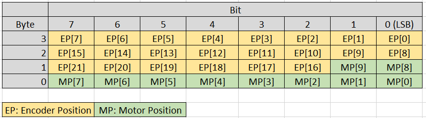
The output buffer size was chosen at 4 bytes. I used bit shifting to achieve this, where the bit allocation can be seen above.
// prepare output buffer to send position and loop index data to python script
// buffer: 22 bits for encoder position (little endian), 10 bits for stepper pos
void update_output_buffer(byte *outputBuffer, long encoderPos, int currentStepperPos) {
  outputBuffer[0] = (encoderPos >> 0) & 0xFF;
  outputBuffer[1] = (encoderPos >> 8) & 0xFF;
  outputBuffer[2] = (encoderPos >> 14) & 0xFC | (currentStepperPos >> 8) & 0x03;
  outputBuffer[3] = (currentStepperPos >> 0) &0xFF;
}
As I restricted the motor position to be between -300 to 300 steps (180° motion range at quarter-step), I knew that I only required 10 bits to fully represent this range. Since the encoder position value is large, I allocated the remaining 6 bits in the motor position buffer to store more encoder position data.
Input Buffer
The input command was the acceleration value of the motor, which was bounded between -20k to 20k. This could be represented fully within 2 bytes of data.
Resetting
Encoder Reset: As discussed above, the encoder position value is very large and can technically keep going to infinity provided the pendulum is swung constantly. Hence, an encoder reset command was implemented.
This was done by sending an input command value larger than 20k (32766). On receiving this command, the encoder would halt for 20 seconds to allow the pendulum to come to rest, before resetting the encoder to 0.
Motor Reset: After each episode ends, the motor position must be reset back to the original 0 position in preparation for the next training run. Hence, similar to the encoder reset, a command input value was defined (32767), triggering the robot to reset its motor position.
Environment
As I needed the robot to be compatible with existing reinforcement learning packages, I followed the gymnasium environment Class structure to ensure that my robot could interact seamlessly with the model. Since I used Stable-Baselines3 (SB3) for this project, I followed their custom environment guide when building the environment. Below are the essential functions implemented:
_setup()
This function is called at the very start of training and after every reset. The function sends a matching authorization string to and from the Arduino to ensure that both are able to “hear” other clearly. Afterwards, the first position value of the motor and pendulum is received from the Arduino. This is crucial, as velocity cannot be calculated without an initial position value.
step()
The step function is called every time the RL model makes a decision. The function receives the action input from the model and outputs the observation array, along with whether the environment has been terminated or truncated. This function is the connecting bridge between the robot and the RL model, where I used pyserial to enable serial communication between the two.
Unlike simulation environments that respond instantly to the RL model and stop moving when the RL model is making its decision, training on a real environment means that any slight difference in latency between the RL model sending the command and the robot executing it would affect the robot’s performance. This is a problem, as throughout the training process, the speed of the model can change dramatically based on the computation with each step. Hence, I used the command self._enforce_control_frequency() to set a fixed control frequency for the robot.
The motor and pendulum velocity readings were calculated by comparing their positions in the current and last observations, along with the time between the observations.
reset() and close()
As discussed above in the control section of the robot design, a reset command is sent to the robot after every episode to reset the motor back to its zero position. The encoder is also reset during this process. Note that the encoder cannot be reset during the training itself, because the pendulum must come to a complete stop in the vertical down position for the reset to be done correctly.
After resetting the position, the environment is setup once more by calling _setup().
The close function is implemented at the end of the entire training cycle, but in our case, we simply use it to call a final reset().
Conclusion
Combining everything together, I was able to get the robot to perform reasonably well (but not perfect!), keeping the pendulum upright for almost a minute. Using the tensorboard logging callback in our code, the first 200k timesteps of training a robot from scratch can be seen below (first 100k in red, second 100k in blue):
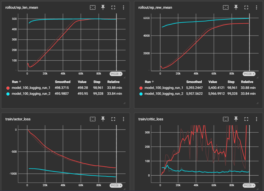
The graphs indicate that the model is converging well at 200k timestep. From the rollout/ep_len_mean graph, we can observe that the robot learns to stay within the allowed motor position range in the first 100k timesteps. The rollout/ep_rew_mean also reflects the robot converging towards maximising its reward, where there is an upward trend even at the end of the 200k time steps.
Learning Points
This project was truthfully much more challenging than expected. Setting up the environment and getting everything to play nice with each other was challenging, along with trying to squeeze out as much performance as possible from the robot. However, I learnt to apply key concepts like state machines and bit shifting that I learnt from my first year at university, which felt quite rewarding.
This project was also a deep dive into reinforcement learning and its challenges, where I have a much better understanding of how reinforcement learning environments are designed, how to better apply the different types of models available (DQN, PPO, SAC, etc.), and how the different parameters affect the model’s performance (gSDE, episode length, reward weights).
Further Improvements
Although the robot is performing reasonably well, I aim to get the robot to be able to keep the pendulum balanced indefinitely. I see potential in the following areas for improvement:
- The Arduino Nano is limited in its computing speed and communication speed and is a potential bottleneck for the system. I hope to replace it with a more capable microprocessor like a Jetson Nano or ESP32. With this speed improvement, I hope to achieve a higher control frequency to make the robot more responsive.
- Further tweaking of the model parameters such as episode length or reward weights could help the model be able to explore more efficiently and converge better. I was looking towards using the weights and biases sweep with wandb.ai on Furuta Pendulum simulations to optimise the parameters.
- Further optimisation of the code could be done. I profiled the code with snakeviz previously to optimise some of the functions. However, much of the computation time is spent on the model training
- I am also looking to run the model on a more powerful machine, which could also help train the model at a higher control frequency.